
О PCA-разложении в задачах с волновым аттрактором
О PCA-разложении в задачах с волновым аттрактором

Аннотация
Волновые аттракторы, представляющие собой особые гидродинамические течения, образующиеся в результате самофокусировки внутренних или инерционных волн, являются довольно сложной задачей как с точки зрения вычислительной гидродинамики, так и визуализации из-за волновой неустойчивости, вызванной увеличением амплитуды волн. В связи с этим использование методов понижения размерности, таких как метод главных компонент (PCA), представляет особый интерес и в последнее время широко применяется к гидродинамическим данным таких потоков, особенно в численных исследованиях. В данной работе мы обсуждаем особенности применения PCA к течениям с волновыми аттракторовами, методы их ускорения и сходимость для этого класса задач.
1. Introduction
Internal waves play an important role in climate formation
, , vertical mixing in the oceans , and seabed erosion . Under certain circumstances , internal wave may self-focus, forming a coherent structure called a wave attractor , . The latter studies showed that wave attractors tend to produce the secondary waves , , with the instability being developed of the Triadic Resonance type , , , . For the real water reservoirs, more typical is the elongated basin form , , . The investigation of wave attractor in large aspect-ratio domains , , (those whose horizontal sizes are larger than vertical ones) revealed that such flows produce more (respectively, small-aspect-ratio ones) intensive instability, whose type is parametric subharmonic.The attractor has been studied both experimentally
, , , and numerically , , , ; in recent years, the latter approach prevails , , , . The wave nature of the attractor structure and the instability make the researcher seek advanced methods for wave attractor visualization. The more popular become mode decomposition methods like Principle Component Analysis (PCA) , . Mainly, the most significant modes are considered for the attractor subflow, the rest are neglected as parts of instability; only considers minor modes. This force to investigate the convergence of such methods and to evaluate their accuracy.In this article, we provide a PCA-decomposition research applyingly to several wave-attractor problems. The questions of numerical application, methods, acceleration and emode number are discussed.
2. Research methods and principles
2.1. Numerical setup
During this research, wave attractor flows were investigated numerically, in 2D formulation, using high-order spectral-element software Nek5000. The numerical approach was validated in
, , , comparing with the experiment results, the 2D approach was verified in , , , . The work provides a cross-validation between the current set-up in Nek5000 and the simulation in OpenFOAM (solver mulesQHDFoam). However, the latter approach is mostly aimed to the large-scale structure rather than instability reproduction, while the small-scale modes are usually investigated with POD ; thus, the high-order Nek5000 package known to reproduce the instability structure correctly was selected.To simulate an attractor flow, the following equations were used:
Navier-Stokes equation in Boussinesq approximation:
salt transport equation:
The salt transport is obligatory since the startification is required for the internal wave propagation.
The last equation is the continuity one for the incompressible fluid:
In the incompressible flow in Bousinesq approximation energy conservation equation is not required. Here the following notations were used:
During the simulation, we used the constant uniform viscosity value

Figure 1 - Geometry sketch
The simulation was run from the steady liquid (i.e., initial velocity condition was zero), initial salt density distribution was linear:
so that buoyancy frequency was constant. The flow was exited by a moving-wall wave maker
situated on the top side of the area; the corresponding boundary condition wasThe amplitude
For
The high-order spectral element meshes used for the simulation are represented in Figures 2–3. The elements shapes can be arbitrary convex quadrilaterals; the orthogonality in this method is not required.
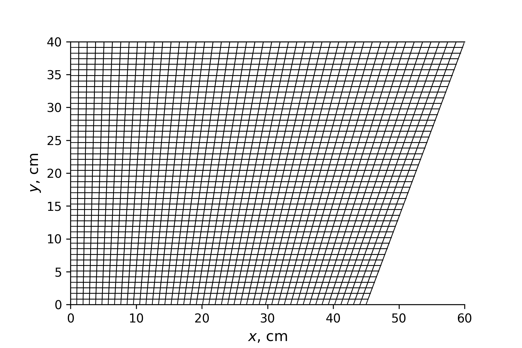
Figure 2 - Low-aspect ratio domain mesh 48x48 spectral element
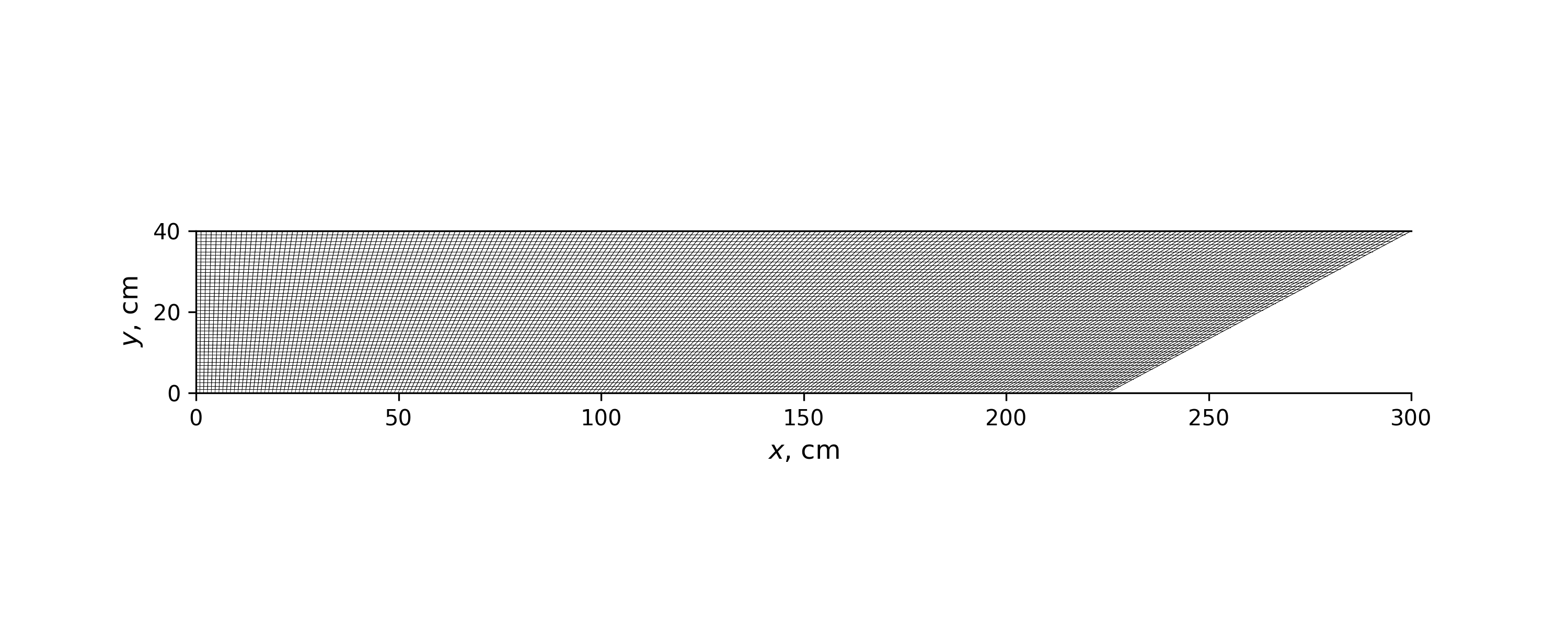
Figure 3 - Large-aspect ratio domain mesh 208x48 spectral elements
Principal component analysis represents the spatio-temporal variable
where spatial modes
To calculate modes, the eigenvectors of the covariation matrix
Such a procedure saves computational costs (time and memory).
Nevertheless, the direct SVD calculation can also be time-costly, since it calculates all the singular values and vectors (their number corresponds to the number of spatial points of the grid). For the amplification, several numerical methods are used; the most popular are ARPACK and randomized SVD. The first one creates the solution iteratively from the random initial approximation, constructing the Krylov subspace, calculating the required number of the first singular vectors; the latter one projects the original data into a random subspace with the following corrections. All the methods are available in python3 (scikit-learn package).
Despite both of these methods being well-tested and reported to yield results close to the full SVD, the wave attractor flows can have a developed secondary-wave subflow that should be correctly reconstructed, and the convergence of the PCA on these problems was not investigated.
3. Main results
Due to the internal wave focusing, the liquid motion is localized in a specific figure, and the oscillation amplitude increases. Figure 4 represents a typical non-linear regime in the small-aspect ratio domain: the parallelogram-shaped
coherent structure is distorted by the secondary waves. In large-aspect ratio domain problems, this effect manifests more clearly , , .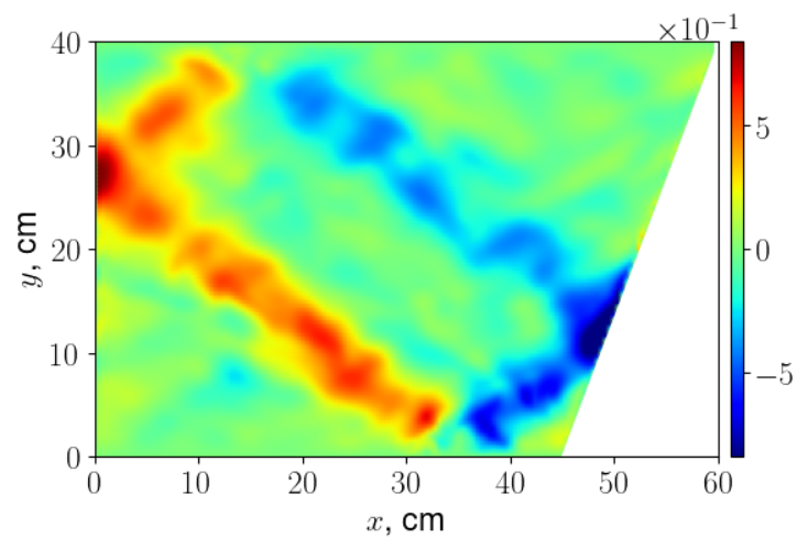
Wave attractor in small-aspect ratiodo main, vy snapshot
colorbar in cm/s
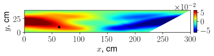
Large-aspect ratio domain problem, initial attractor development befor the instability formation
colorbar in cm/s; black dot is the characteristical point
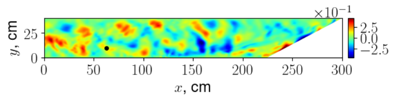
Large-aspect ratio problem, vy snapshot developed non-linear regime
colorbar in cm/s, black dot is the characteristical point
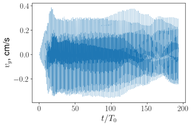
Figure 7 - Temporal behaviour of vy in the point selected
To check the quality of PCA decomposition, full
where the solution reconstruction
where
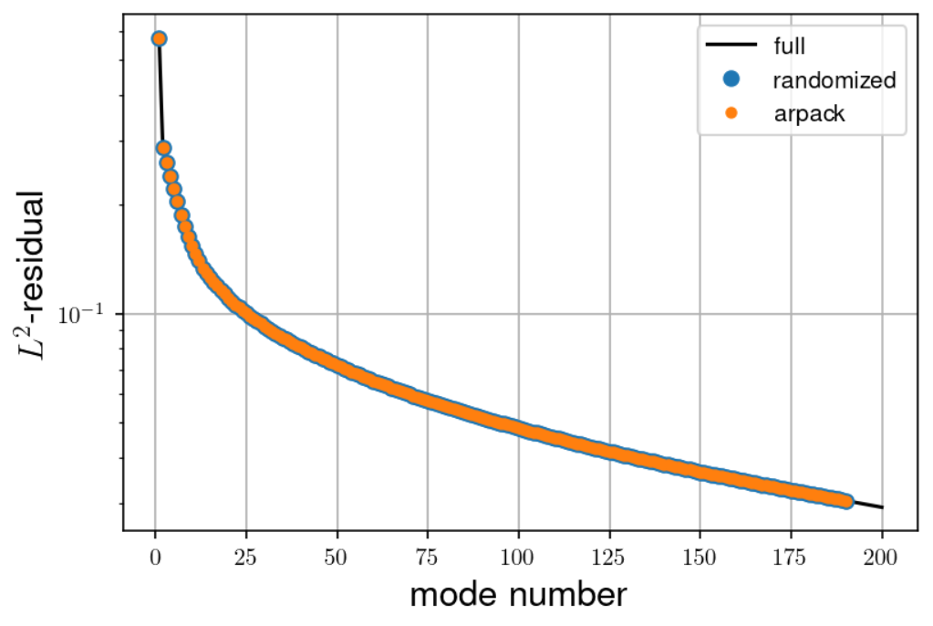
Figure 8 - Residuals in small-aspect ratio problem decomposition
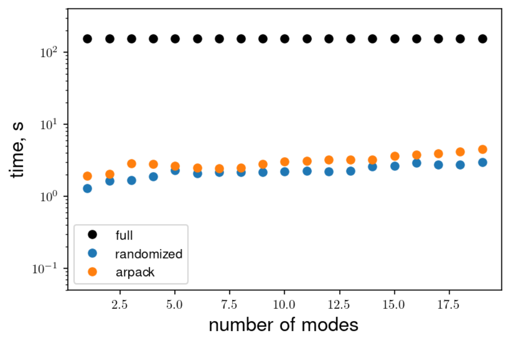
Figure 9 - Execution times for different SVD calculation methods
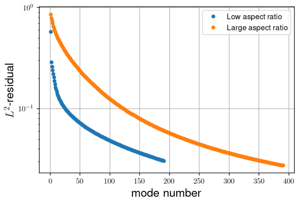
Figure 10 - Comparison of reconstruction residuals for different aspect ratio
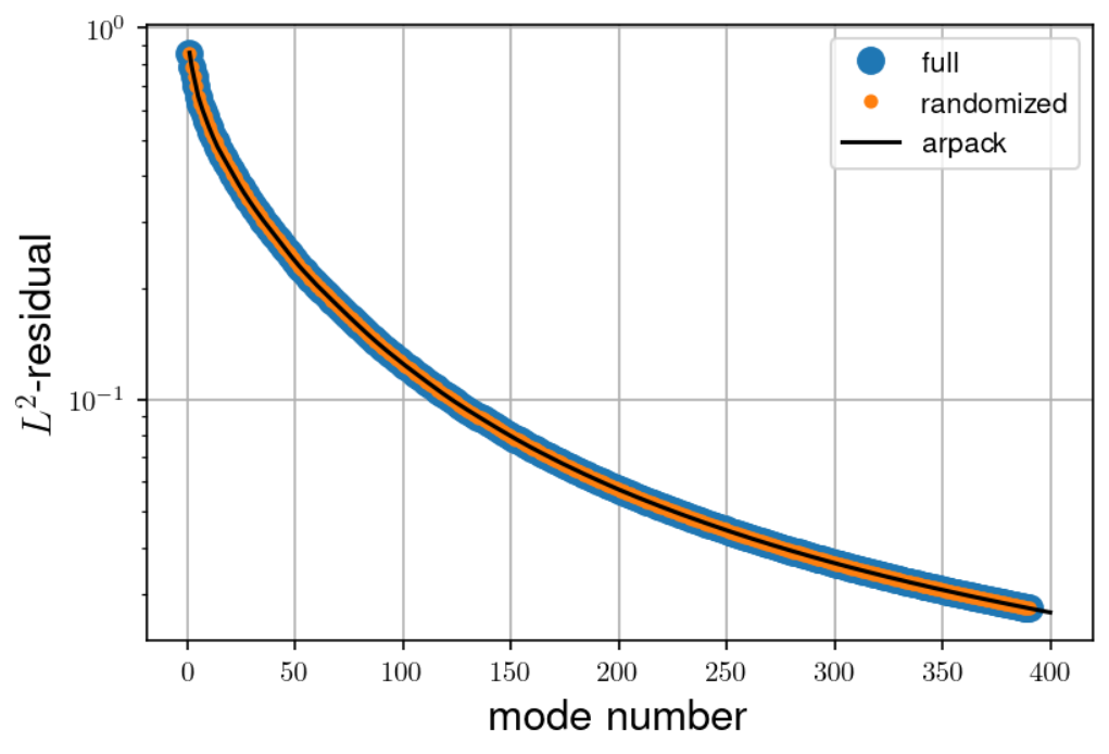
Figure 11 - Large-aspect problem residuals
4. Conclusion
The PCA decomposition was considered for the wave attractor problems. Both full SVD and reduced methods yield the same accuracy of by-mode reconstruction, which allows to use the latter one without significant losses. It was found that their use can accelerate the computation up to 100 times, with the fastest being the randomized SVD approach.
The large-aspect ratio problems demonstrate less residual decrease with the used mode number and thus require more modes for the same accuracy in comparison with the small-aspect ratio problems. This makes the indirect SVD methods application even more preferable.
Withal, PCA method converges slowly and requires about several hundred modes for a precise enough reconstruction, which limits the investigation of secondary waves, forming the instability, with this method.