A methodology review for wave-attractor problems
A methodology review for wave-attractor problems
Abstract
Wave attractors are specific and complex flows, formed by a self-focused internal or inertial waves. In linear regimes they appear as clear coherent structures of a certain shape; in non-linear ones the intensive formation of the secondary waves occurs which distort the coherent structure. Their presence, along with the huge localization of the flow, makes one to select thoroughly the post-processing methods in such flows (including energy characteristic calculation, spectral investigation, visualization etc.). In the existing articles, these methods vary from work to work. The goal of this paper is to consider different method for processing the flow data applied to wave attractors in order to compare their particularities and to reveal the best practice for the further using.
1. Introduction
A wave attractor is a result of internal/inertial waves self focusing
. The main feature of the wave attractor is the huge ratio between the amplitude on it and that of the wave-maker , , which causes the wave instability at the respectively small wave-maker amplitudes . Such flows are characterized by the great energy accumulation and specific spectrum caused by the wave instability appeared in these flows which are frequently calculated and investigate qualitatively as well as quantitatively, which means they should be, on the one hand, precise enough to reflex the complex structure of the flow, and on the other hand, be general-purpose to require minimal setup and to have clear requirements to be applied (such as signal point number etc.). However, there appear to be the variety of methods, changing from work to work, that requires the thorough investigation and comparison of these technical methods themselves.In this investigation, the corresponding review of the methods used for wave-attractors flow processing will be conducted. For this purpose, the numerical simulation result will be used following
, , , ; 2D formulation, whose accuracy is shown in , , , , is applied to save computational resources.2. Research methods and principles
The simulation is conducted in open-source package Nek5000
, using spectral-element approach for high-order simulation, which is validated for wave-attractor flow simulation , , , . For the internal waves propagation, the stratification is required which is created by dissolved salt stratification in water. The following system of equations is solved:These are Navier-Stokes equation in Boussinesq approximation, dissolved salt transport and continuity equation. Here
For the focusing, internal waves require a slope
; thus, the minimal geometry for wave attractors study is a trapezium, as shown on Fig.1. This study will mainly use the trapezium-shaped domain except the case with mid-depth plateau, whose geometry will be shown in what follows.

Figure 1 - Domain principle outline
The other specific parameters (like viscosity, startification profile, wave-maker amplitude and frequency etc.) are varied from case to case; the specific values can be found in the article describing each particular case (the link will be provided in the corresponding sections).
3. Main results
3.1. Energy Local Average Calculation
Kinetic energy is one of the most frequently appearing characteristics when discussing wave attractors. Its popularity is based on its huge values typical for this flow type.
The total kinetic energy is defined as
where
In wave attractor flows, the
Since both energy and relative energy differ to a constant, their behaviour is the same, and the principles considered in what follows are applicable to both of them to the same extent.
The energy behaves specifically in time: at the formation process it grows, that reach the saturation, after which begins to "noise" (it is conditioned by the additional harmonics from the secondary waves). The energy has a tendency to oscillate even in a linear regime
, , it occurs due to a presence of the standing waves along with the running ones.To describe the system, the local average value is used (the oscillations are excluded); however, because of the rapid increase at the beginning and non-linear oscillations, the average obtaining becomes a non-trivial problem. Local average is required to maintain the following principle properties: to start from zero (as the real kinetic energy) and to not start to oscillate while the instability develops.
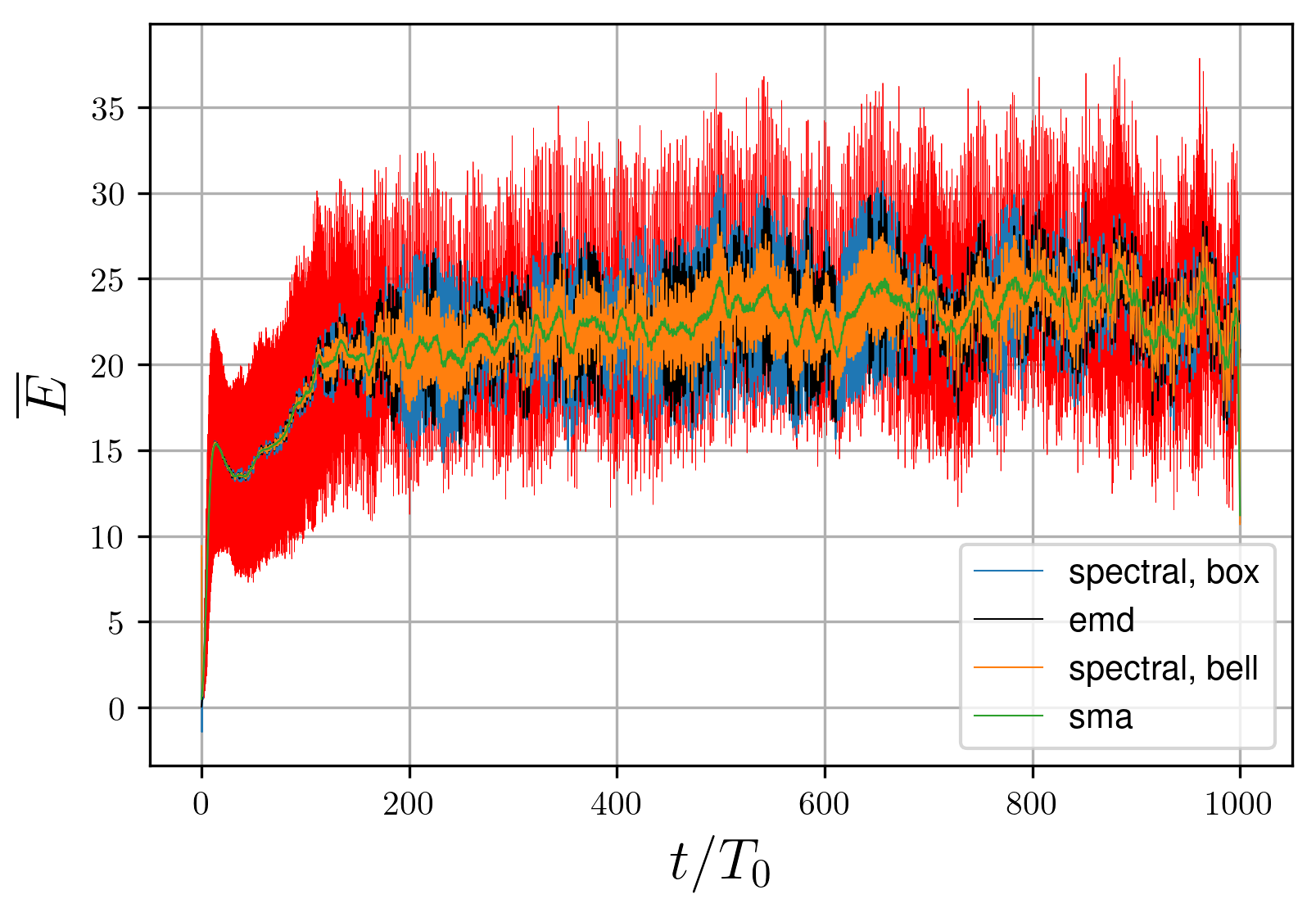
Figure 2 - Energy behaviour in a non-linear regime (red) with different methods of the local average estimation
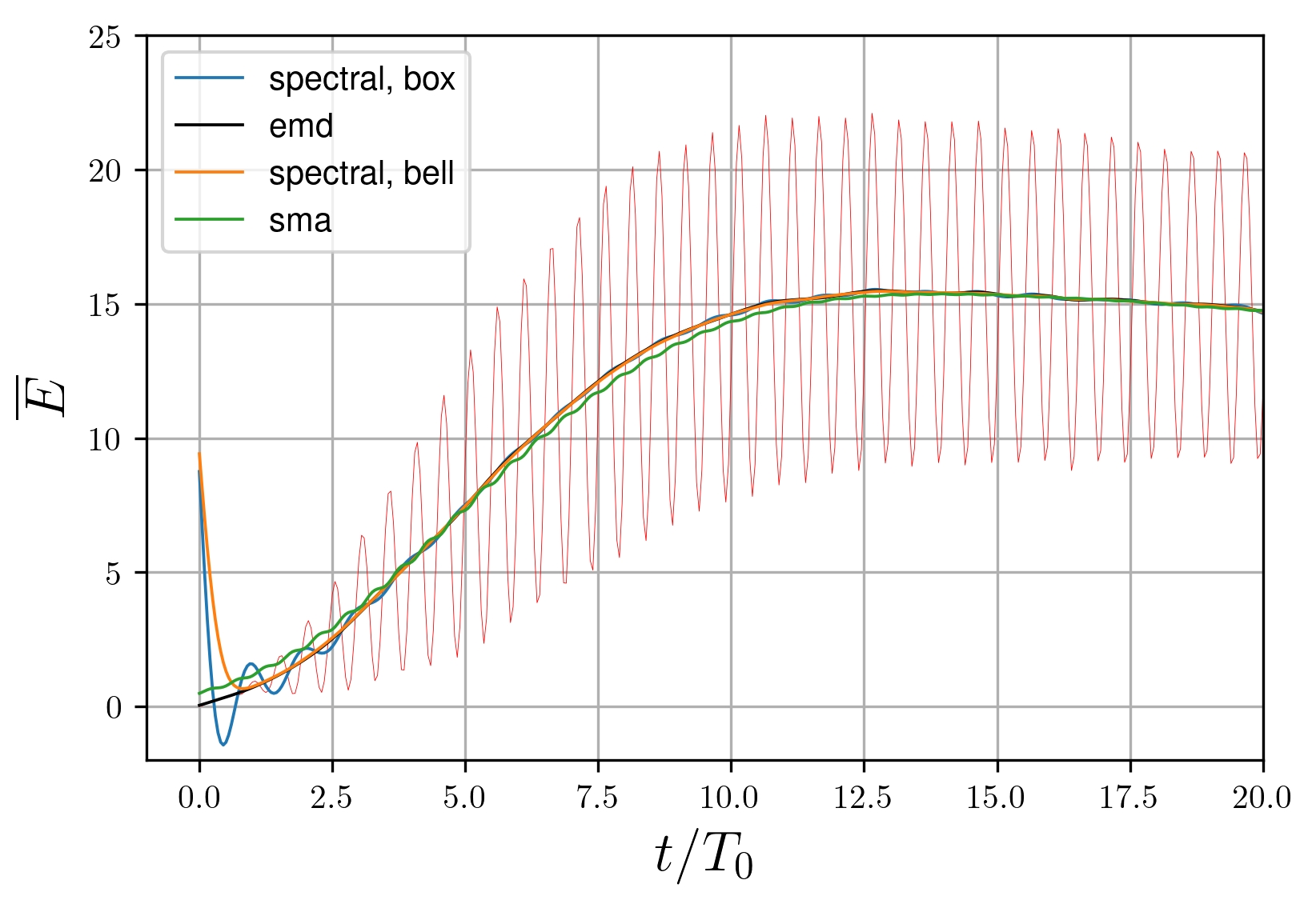
Figure 3 - Energy at the attractor fomation time range
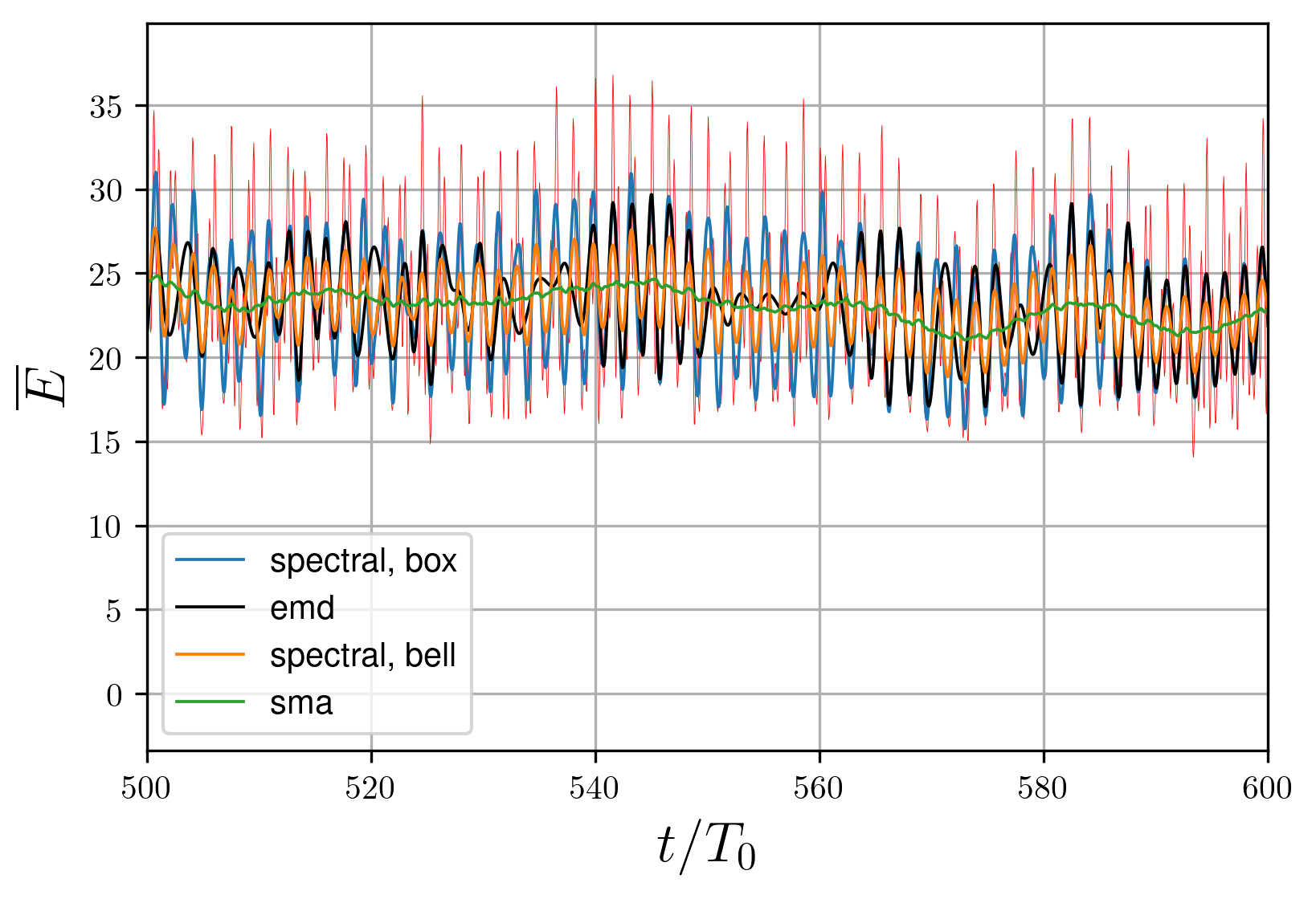
Figure 4 - Energy at the developed instability
The method does not require special fitting and is governed by the number of filtration modes. The increase of
The next idea is the spectral filtration; the higher frequencies of the spectrum are suppressed, and then the inverse transform is conducted:
The different filter action on a real energy spectrum is represented on Fig. 5; the "box" filter is
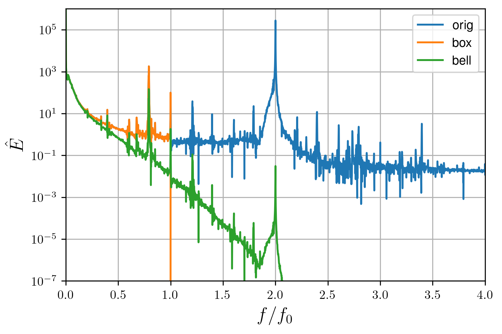
Figure 5 - Energy spectrum with different filtartion
where
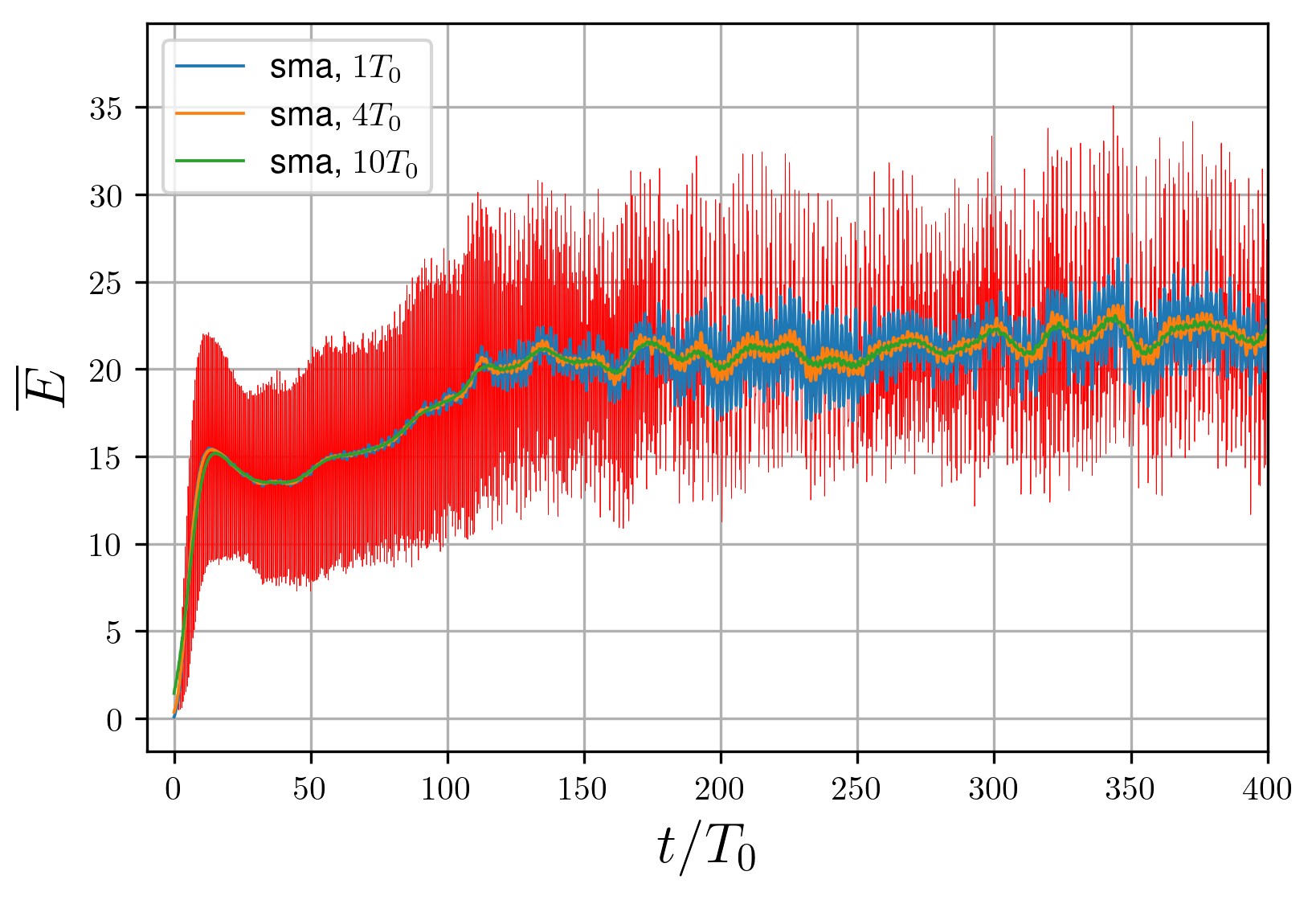
Figure 6 - Energy local average calculation with simple moving average
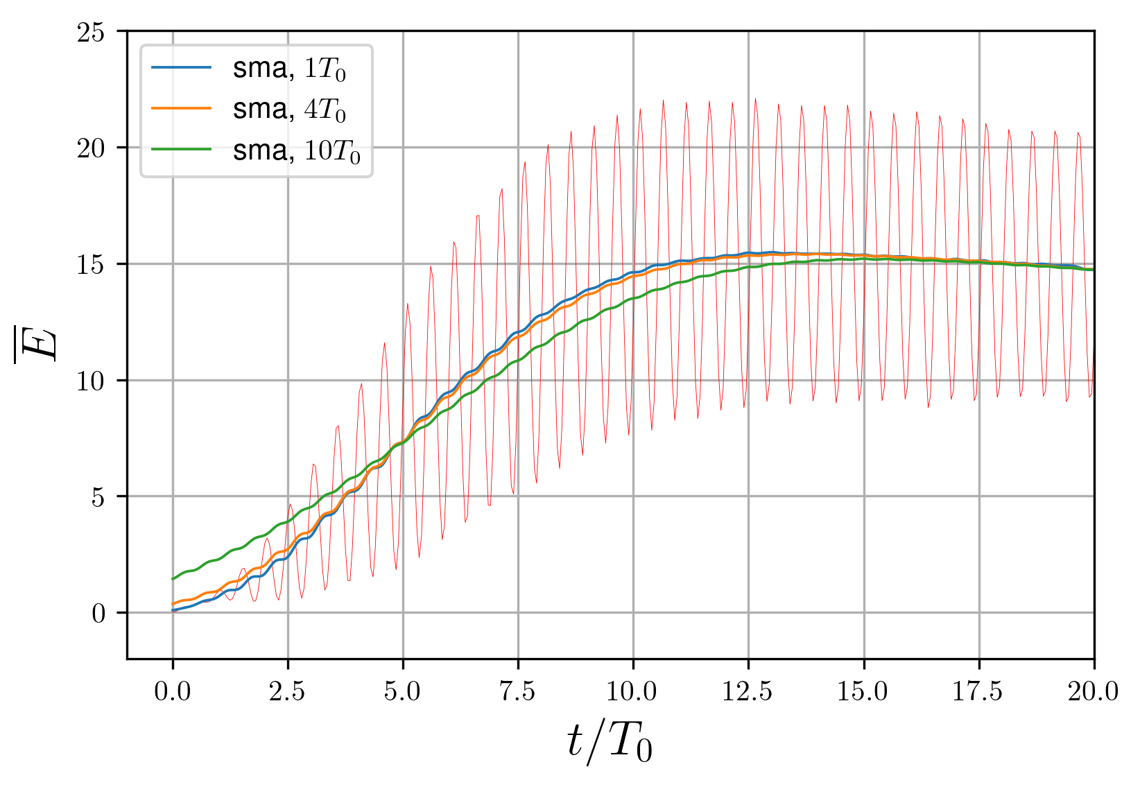
Figure 7 - Moving average action at the attractor formation time: the window width influence
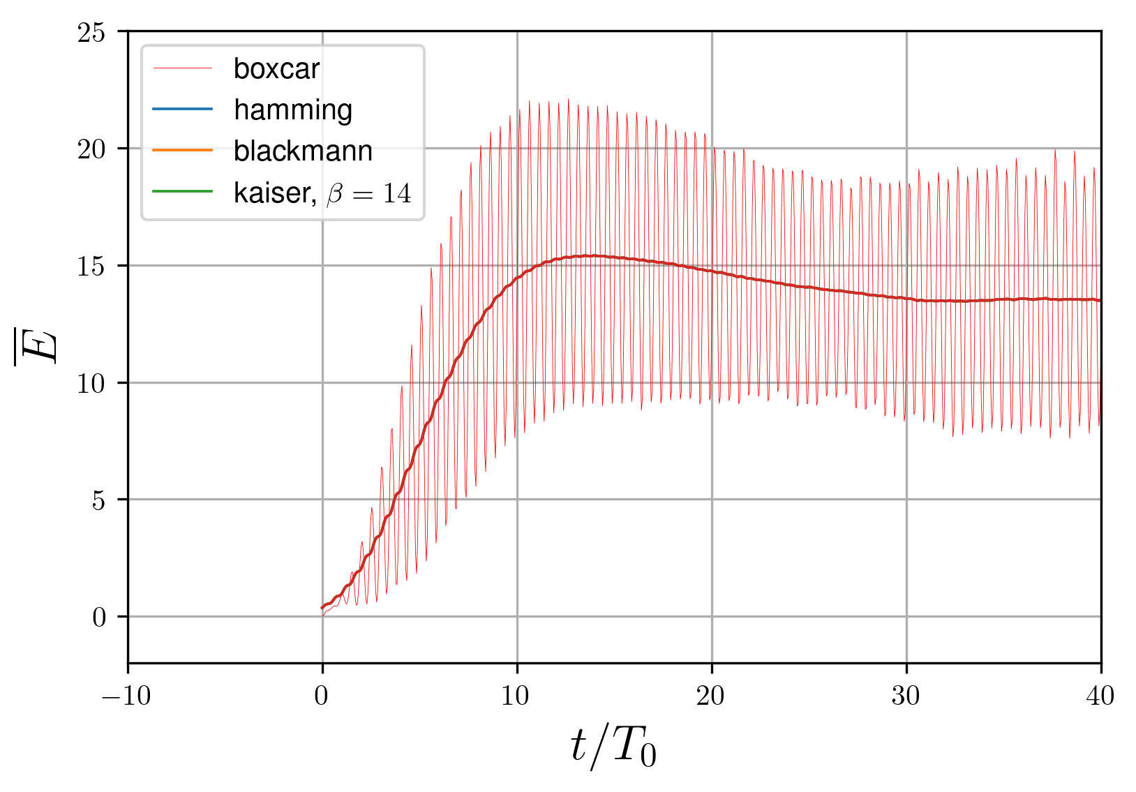
Figure 8 - Window influence on the moving average calculation: formation times
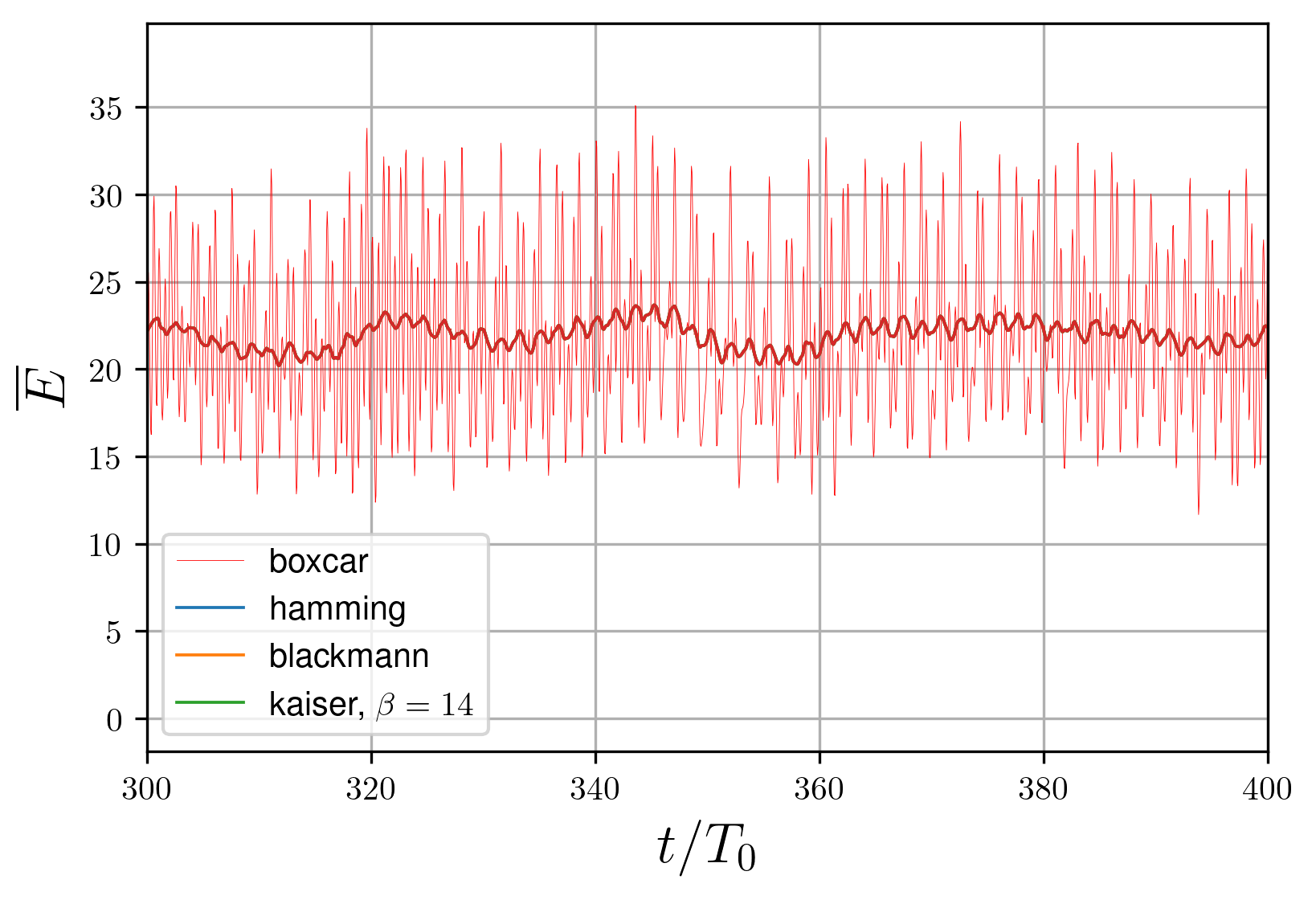
Figure 9 - Moving average calculation: developed instability
The temporal spectra, while calculated for an attractor flow, are investigated in a point; as a representative point, the attractor's ray middle (Point 4 on Fig. 10) is usually considered
, , , .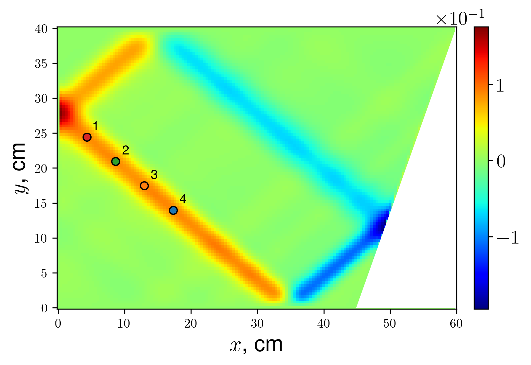
Figure 10 - Liner attractor regime, vy snapshot and spectrum calculation locations
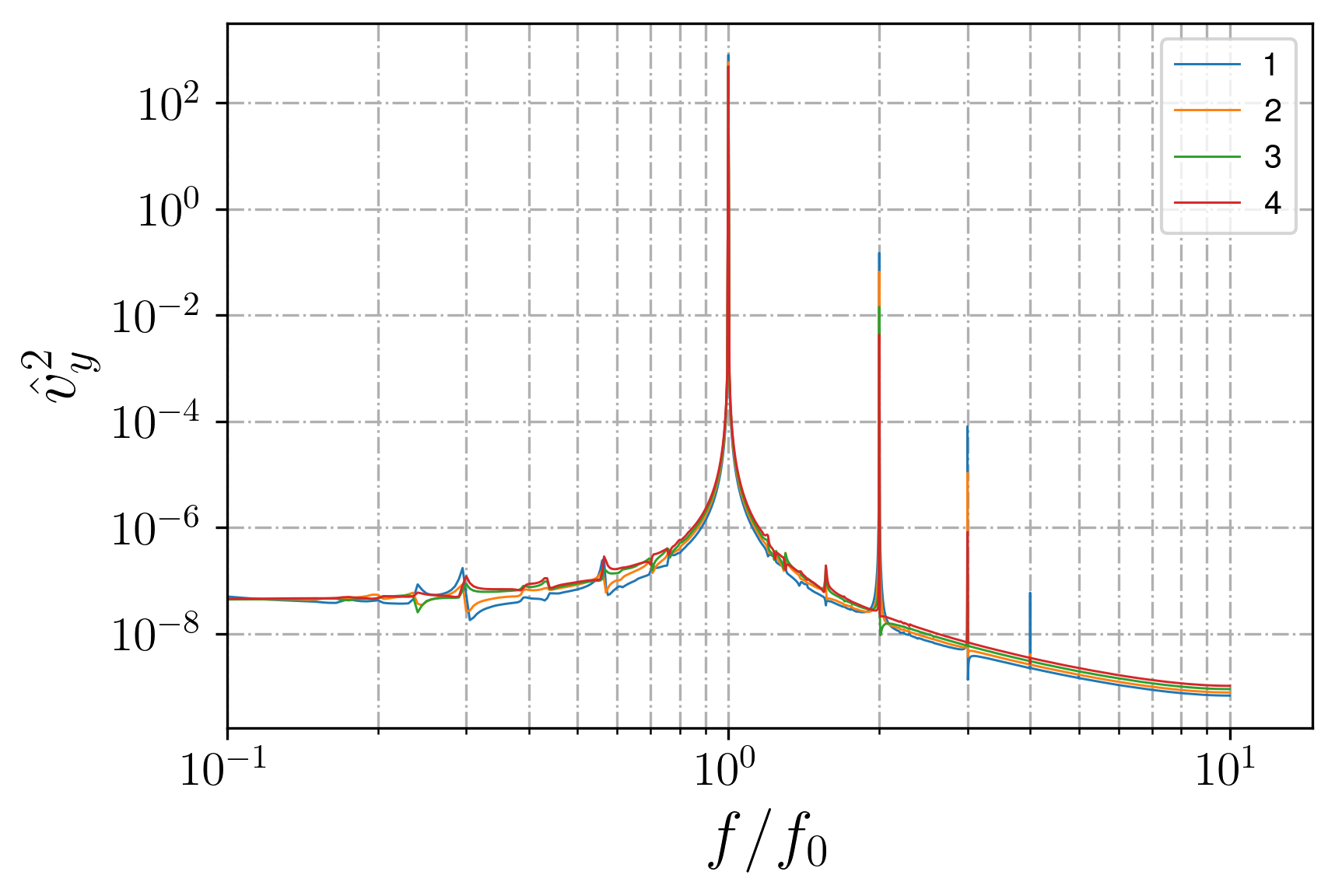
Figure 11 - Linear attractor regime, spectra in different locations
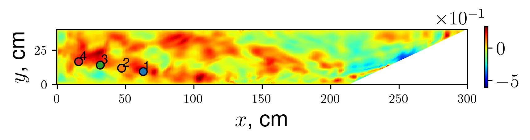
Figure 12 - Non-linear attractor regime in a large-aspect ration domain, vy snapshot and spectrum calculation locations
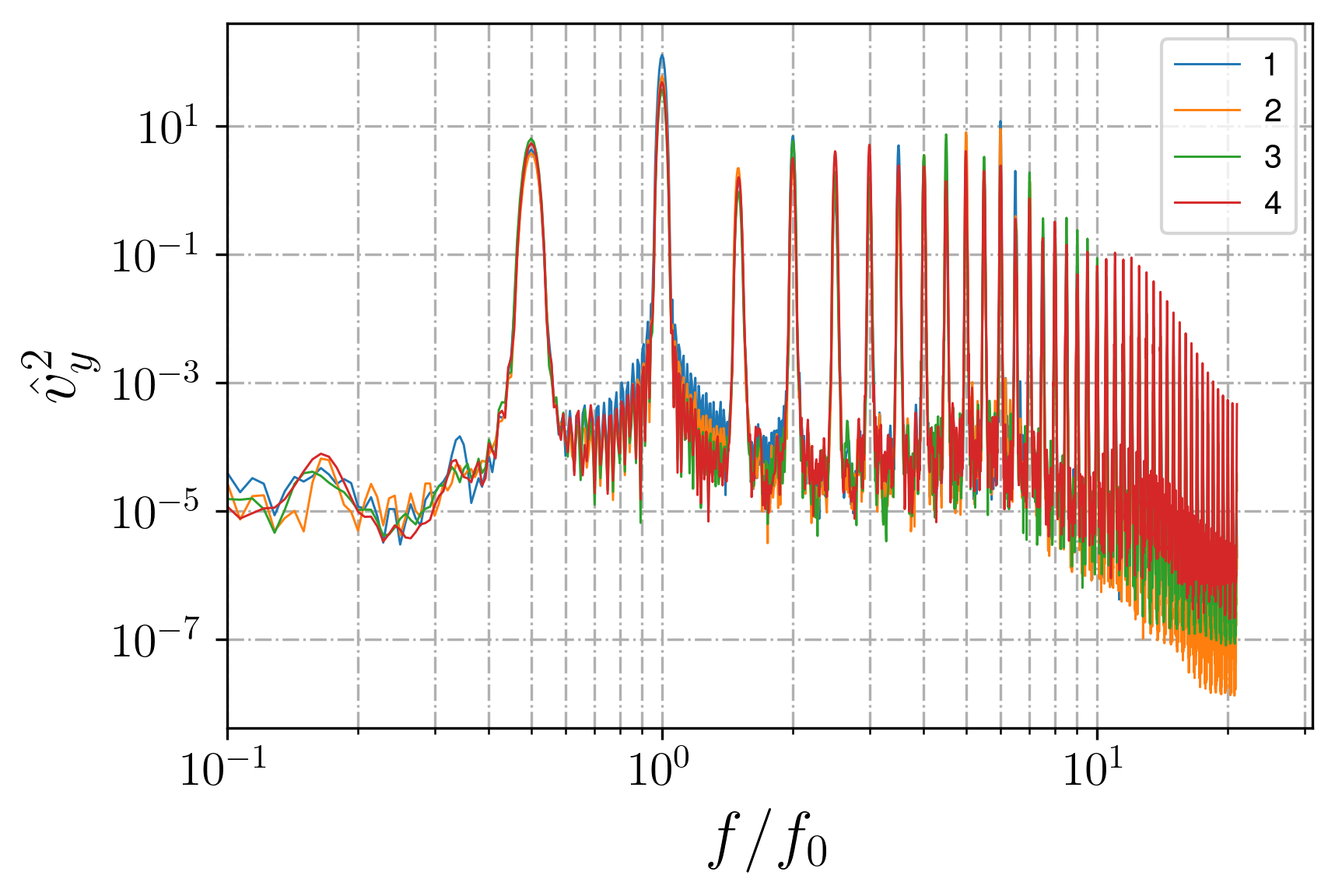
Figure 13 - Spectra in different locations for large-aspect ratio attractor
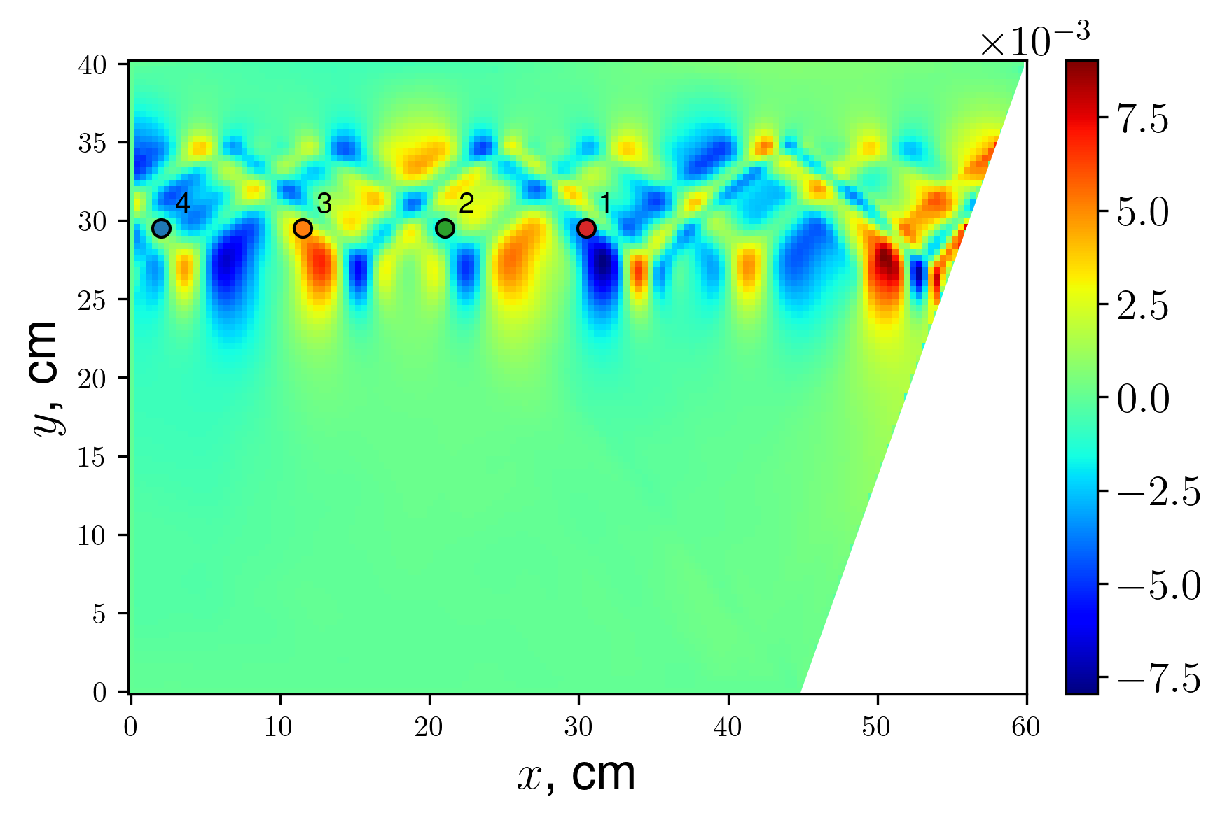
Figure 14 - Attractor in a layer, vy snapshot and spectrum calculation locations
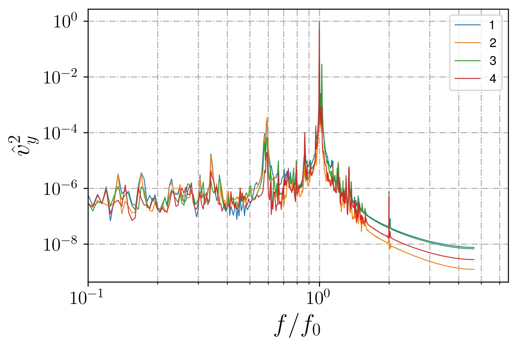
Figure 15 - Attractor in a layer spectra in different locations
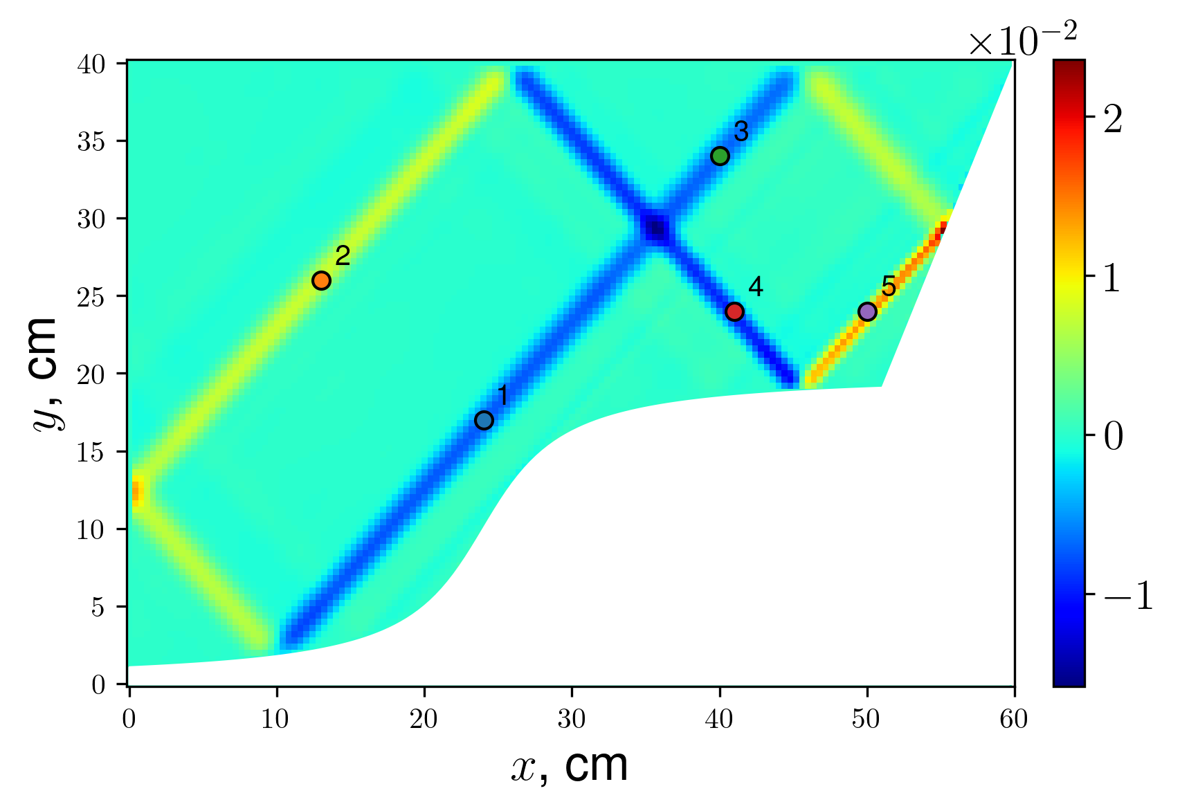
Figure 16 - (2,1) linear-regime attractor in a domain with underwater plateau, vy snapshot and spectrum calculation locations
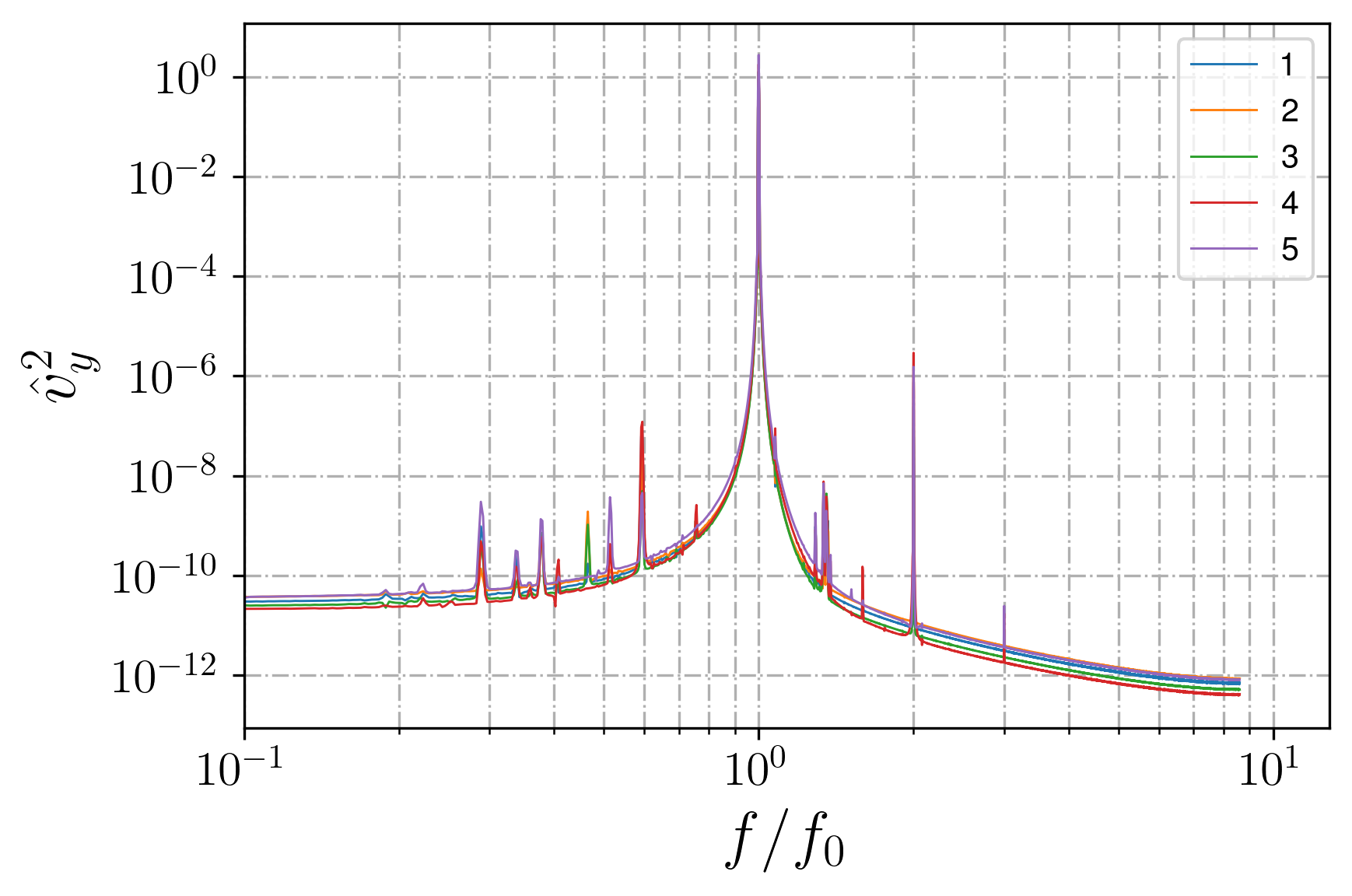
Figure 17 - Spectra in different locations for attractor in basin with underwater plateau, linear regime
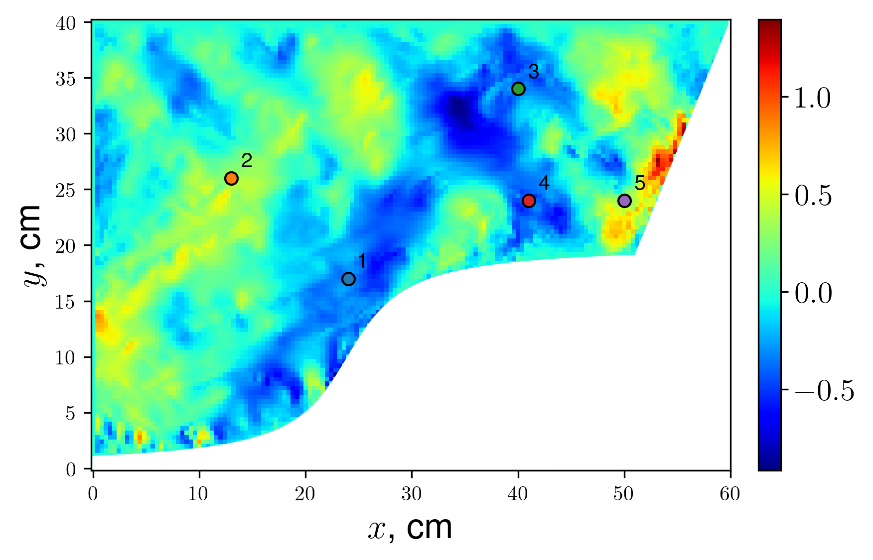
Figure 18 - (2,1) non-linear attractor in a domain with underwater plateau, vy snapshot and spectrum calculation locations
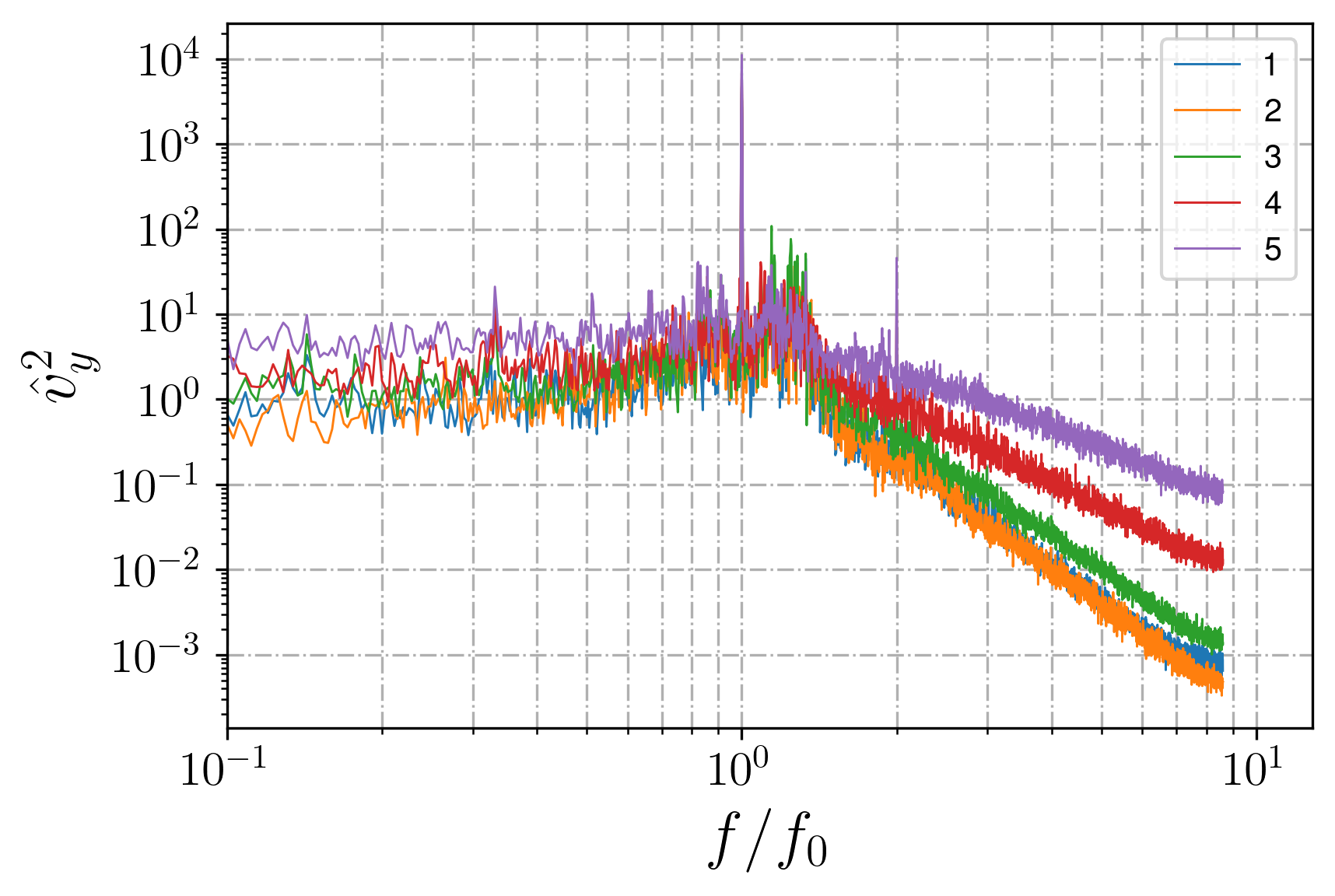
Figure 19 - Spectra in different locations for attractor in basin with underwater plateau, non-linear regime
To improve the spectrum, windows are often applied. There is a set of windows most frequently used (for normalized window range from 1 to -1):
In fact, they can be approximated accurately enough by one of the Kaiser windows with the corresponding
where
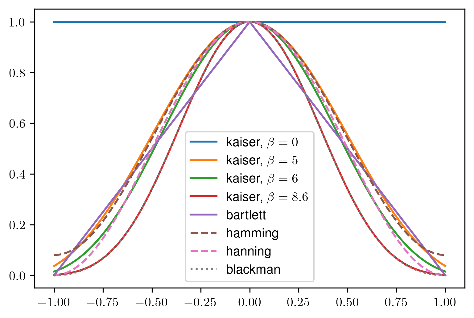
Figure 20 - Different spectral windows
Table 1 - The correspondence between classical window types and parametric Kaiser ones
Window | Similar to, β |
boxcar | 0 |
Hamming | 5 |
Hanning | 6 |
Blackman | 8.6 |
The main consequence of the window using is the reduction of the "background" (the intervals between the peaks) and the revealing of the minor peaks, as shown on Fig. 21. This property is useful when one calculates the ratio between different spectral components; also, the narrow windows eliminate the smooth transition between peak and background, allowing to determine easily the borders of the peak. Note that the background level for Kaiser with high
The other side of the coin is peaks widening, that may affect the minor peaks resolution when triadic resonance instability subharmonics are studied
; however, since the high-frequency part of the spectrum is considered more frequently , , , , the narrow Kaiser windows for such spectral investigations are preferable.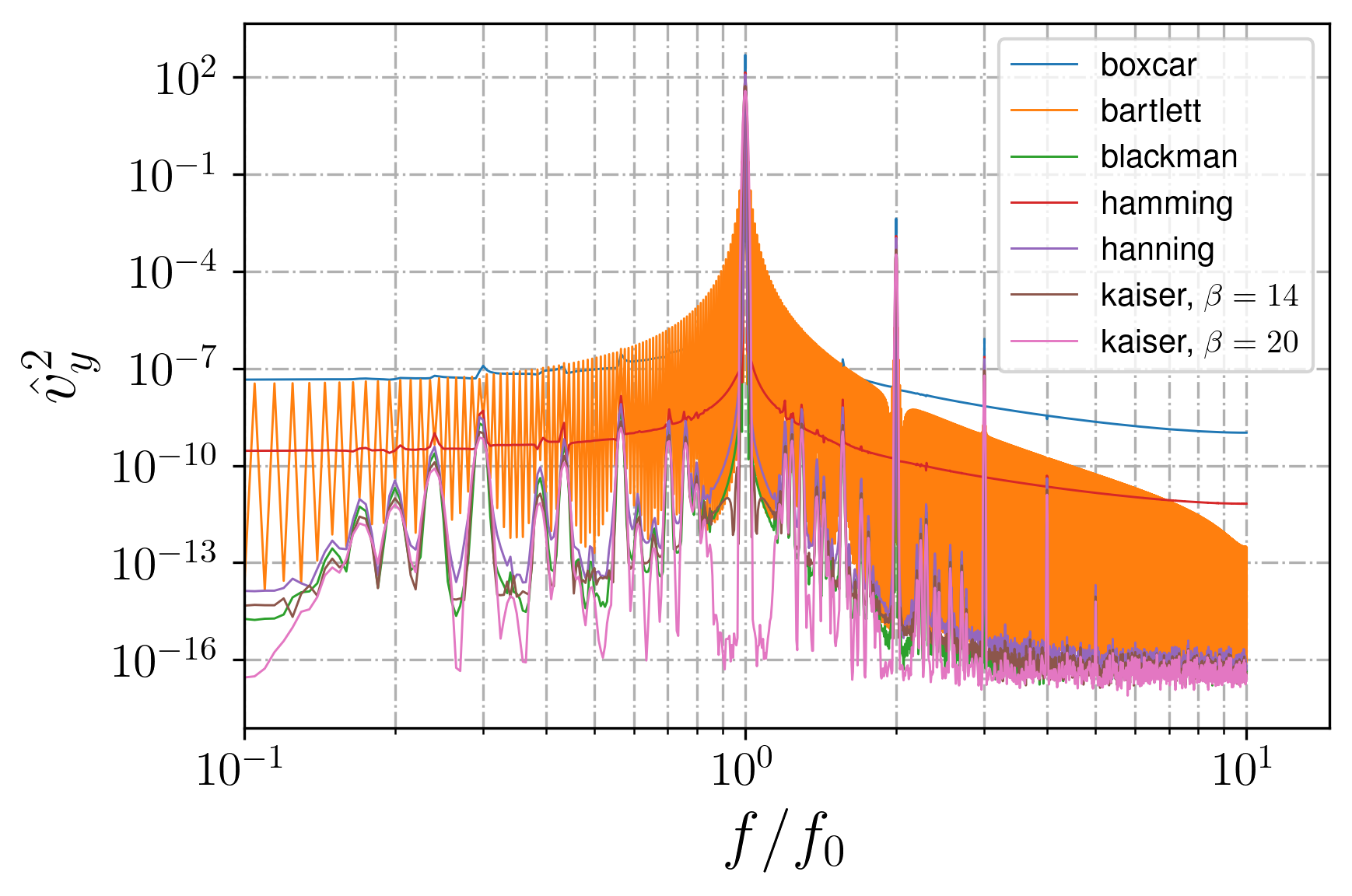
Figure 21 - Wave attractor spectrum calculated using different windows
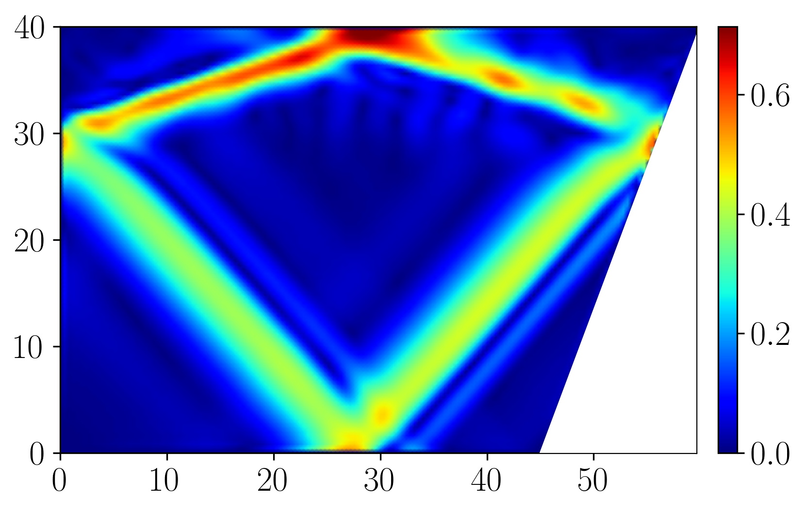
Figure 22 - Wave attractor in two-layered stratification (vy Hilbert transform, cm/s)
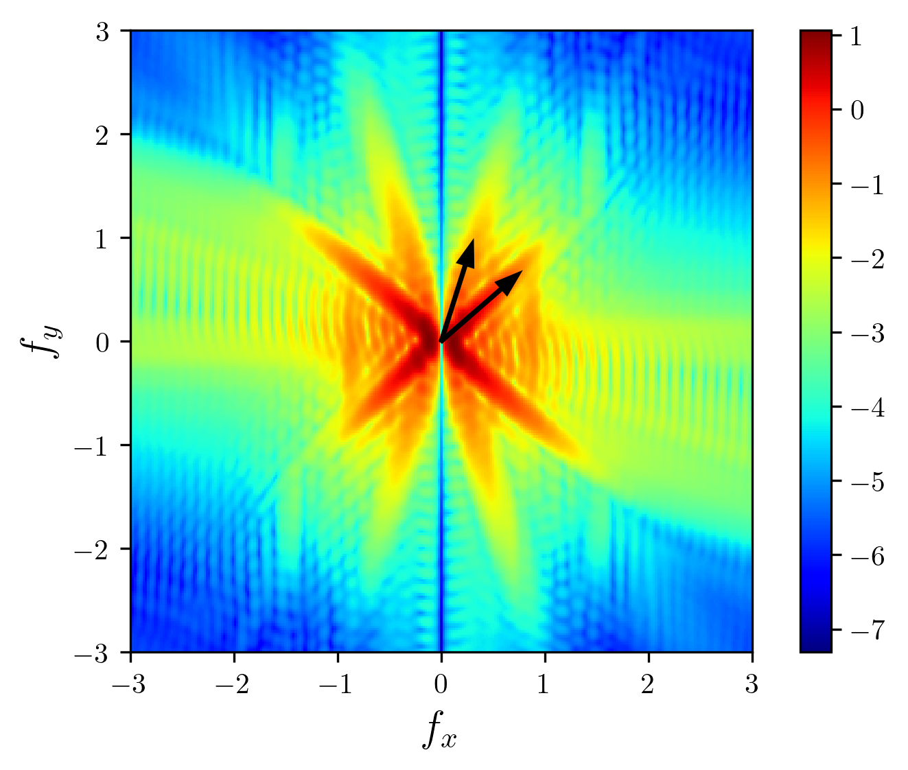
Figure 23 - fx-fy diagram in two-layered stratification, no window
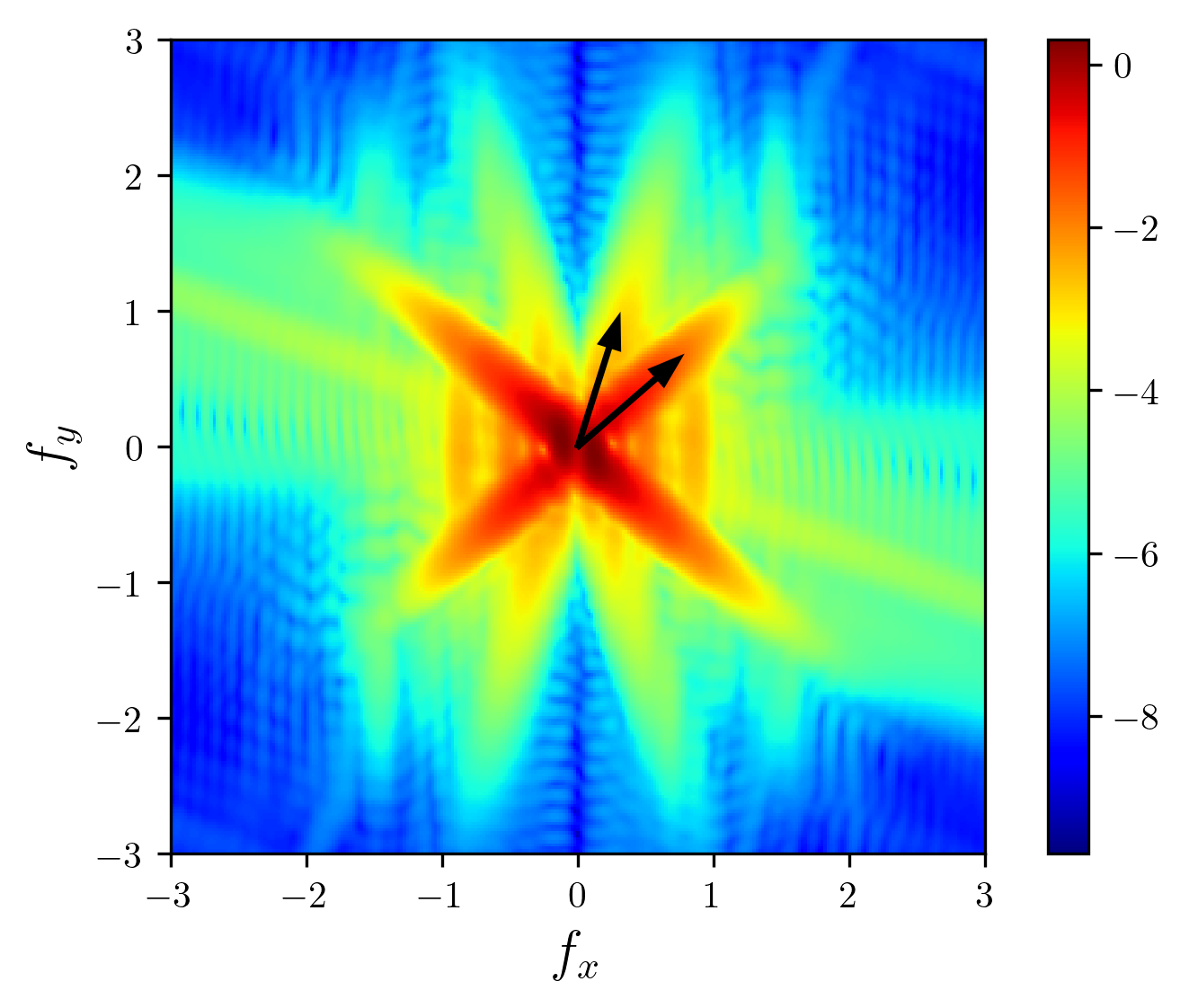
Figure 24 - fx-fy diagram in two-layered stratification, Kaiser window with
β=5
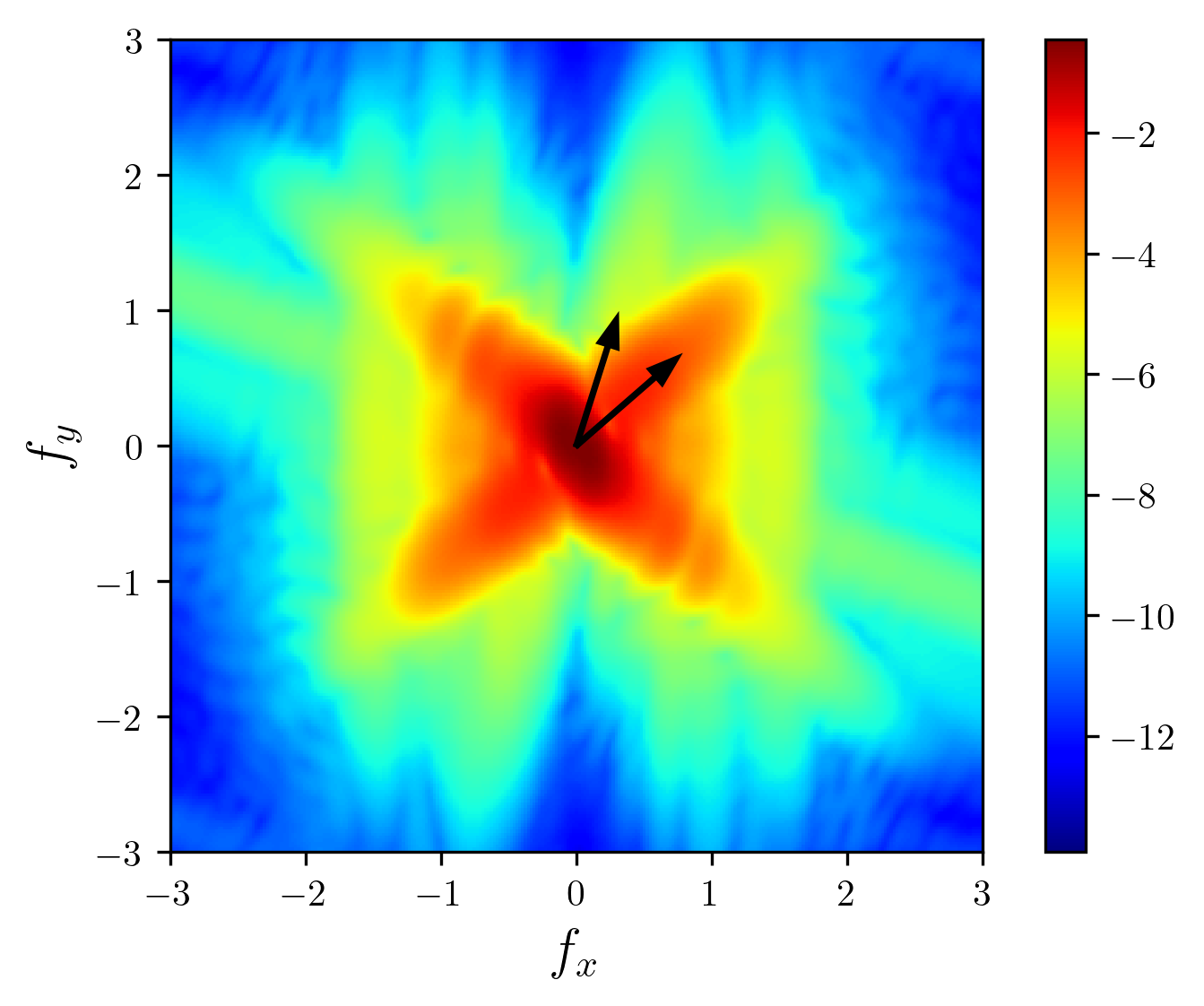
Figure 25 - fx-fy diagram in two-layered stratification, Kaiser window with
β=14
Wave attractor flows are known to have a specific form of the coherent structure, which is frequently considered as a marker of a wave attractor presence, and one strives to visualize it
, , , . The visualization is most frequently done by field map plotting a certain value (whether it velocity component, pressure gradient or Hilbert transform amplitude). The visualization of an attractor is a challenge , , ; thus, the choice of the colormap itself becomes important. The previous investigation seems to have used the colormap provided defaultly by the instrument they use: works , , , uses "jet" colormap from matplotlib.pyplot package, investigations , provides "hot" colormap preset in VisIt software , article plots field maps with "inferno", includes "bwr" and "hot", prefers "fusion". As one can see, there is no unity in the question of the colormap selection; neither there exists a work discussing this problem.The different visualizations are represented on Fig. 26; the plotted is the momentary velocity amplitude. The colormap labels are the same as in the matplotlib package
. For the structure emphasizing (which is most required task), "seismic" or "hot" will be the preferable option. For the background waves resolution, "turbo" is optimal. The "jet" pattern will be a good compromise between them. The other colormaps plot the attractor neither bright nor detailed.The discrete (quantitative) colormaps can also be used for a wave-attractor visualization (Fig. 27). These ones, however, represent the background instability very poorly, which nevertheless may be useful for the structure visualization. "Accent" seems to be better for the structure emphasizing, and none of them reveal the background waves.
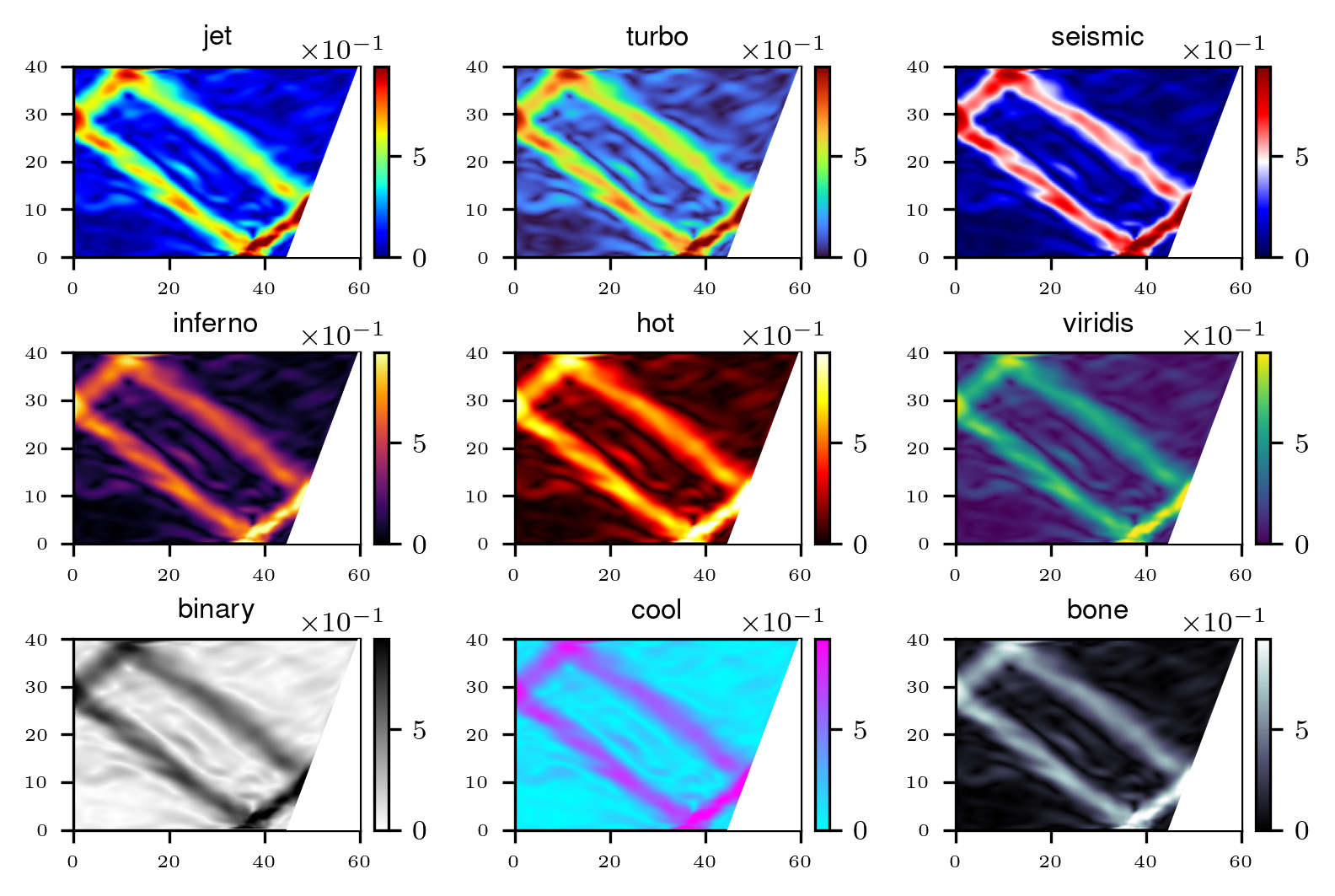
Figure 26 - A wave-attractor in a weakly-nonlinear regime visualization (|v|, cm/s): continuous colormaps
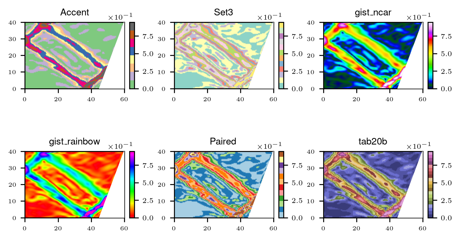
Figure 27 - A wave-attractor in a weakly-nonlinear regime visualization (|v|, cm/s): discrete colormaps
4. Conclusion
Wave attractors as complex flows require a thorough selection of the methods for their processing. In this article, a number of methods were discussed. For the energy mean calculation, the best method was found that is stable for the sharp initial increase as well as for developed instability oscillations. For the spectra, different windows application were discussed and revealed that different windows should be used for spatial and temporal spectra; the influence of the spectrum spatial position is investigated for the different setups, found that it is minimal. Additionally, the field map representation is discussed, the different colormaps are applied, their aspects are shown for the selection in further works.